2009 Group Project 4: Difference between revisions
| Line 370: | Line 370: | ||
3.Hedrich, H., Bullock, G., & Petrusz, P. (2004). ''The Laboratory Mouse''. London: Elsevier Academic Press | 3.Hedrich, H., Bullock, G., & Petrusz, P. (2004). ''The Laboratory Mouse''. London: Elsevier Academic Press | ||
4. Theiler, K 1989. 'The House Mouse'. Springer- Verlag, New York | |||
{{Template:Projects09}} | {{Template:Projects09}} | ||
Revision as of 14:16, 3 September 2009
THE MOUSE
Timeline of Development
- Development of the Mouse Embryo
Day 0 One Cell Egg
Day 1 Dividing Egg. Cleavage of cells has begun. The Day ends with 4 cells present.
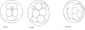
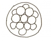
Day 2 Morula
Day 3 Advanced segmentation of the Morula. 16-25 cells within same sized morula.
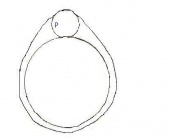
Day 4 Blastocyst formation
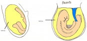
Day 4.5 Implantation and Invasion of the blastocyst into the uterine epithelium
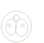
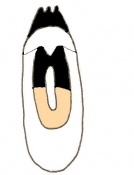
Day 5 Formation of the egg cylinder
Day 6 Differentiation of the egg cylinder
Day 6.5 Gastrulation starts during the period of Advanced Endometrial Reaction
Day 7 Amnion formation
Day 7.5 Neural plate and presomite stage
Day 8 Formation of the first seven somites.
Day 8.5 Rotation of the embryo. The embryo now has between 8 and 12 somites.
Day 9 Formation and closure of the anterior neuropore. There are 13 - 20 somites present in the embryo
Day 9.5 Formation of the posterior neuropore and forelimb bud. There are 21 to 29 somites present and the embryo measures 1.8 - 3.3 mm in length.
Day 10 The posterior neuropore closes and formation of the hind limb bud and tail bud occurs. there are 30 - 34 somites present and the embryo is 3.1 - 3.9mm
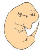
Day 10.5 Deep eye lens indentation occurs. There are 35-30 somites present and the embryo is now 3.5-4.9mm.
Day 11 Closure of the lens vesicle. There are 40-44 somites present and the embryo has reached 5-6mm in length.
Day 11.5 The lens vesicle is completely separated from the surface epithelium. There are currently 45 - 47 somites and the embryo reaches a length of 6 - 7mm
Day 12 First signs of fingers. The embryo is 7 - 9mm in length from crown to rump and there are 48 - 51 somites.
Day 13 The anterior footplate becomes indented and the external ear structure is more defined. The embryo is now 9 - 11mm in length and has 52 - 55 somites.
Day 14 The fingers separate. The embryo has 56 - 66 somites and is 11-12mm in length.
Day 15 The toes separate. At this stage the embryo is 12 - 14.4m from crown to rump
Day 16 The umbilical hernia is repositioned. The fetus now measures between 14 and 17 mm.
Day 17 The fingers and toes become joined together. The skin is wrinkled and thickened and the umbilical hernia has disappeared. The fetus measures 16.5 - 20mm depending on the degree of curvature.
Day 18 Whiskers elongate. The length of the embryo varies between 18 and 23 mm due to the degree of curvature of the fetus.
Day 19 The newborn mouse is between 23 and 27mm depending on the degree of flexure of the body axis


Staging
Mouse embryonic development commences once the female's egg or oocyte has become fertilized by the male's sperm. Mouse development has a gestation period of 19-21 days, and can range in different strains of mice. The development of an embryo can be categorized into different stages including cell number, somite stages and morphology. Link to movie showing mouse embryo [1] The most common method of staging is by Theiler (1989) which categorizes mouse development into prenatal and postnatal stages consisting of 26 and 2 stages respectively. Downs and Davies (1993 ) have also established a method of staging the mouse development based on morphological changes. Link to Downs and Davies [2]


| Theiler Stage | Embryonic Age in Days Post Coitum (dpc) | Stage Characteristic | Cell Characteristics | Zona Pellucida | Location | |
|---|---|---|---|---|---|---|
| 1 | 0-0.9
(range 0-0.25) |
One-celled embryo (fertilized) | One cell | Present | Ampulla | |
| 2 | 1
(range 1-2.5) |
Dividing egg | 2-4 cells
- 1st cleavage after 24hrs |
Present | Travelling down oviduct | |
| 3 | 2
(range 1-3.5) |
Morula (early to fully compacted) | 4-16 cells | Present | Oviduct. Usually near utero-tubal junction. | |
| 4 | 3
(range 2-4) |
Change from Morula to Blastocyst
-Intra-cellular matrix present -Blastocoelic cavity evident |
16-40 compacted cells
-Inner cell mass -Outer layer of trophectoderm cells |
Present | Uterine lumen | |
| 5 | 4
(range 3-5.5) |
Zona free Blastocyst (hatching) | Blastocyst is ready to implant as surrounding cell layer of zona pelludica is lost | Absent | Uterine lumen |
Dr Mark Hill 2009, UNSW Embryology ISBN: 978 0 7334 2609 4 - UNSW CRICOS Provider Code No. 00098G
Link to ultrasound of mouse embryo [3]
| Theiler Stage | Embryonic age in Days Post Coitum (dpc) | Stage Characteristic | Cell characteristics | |
|---|---|---|---|---|
| 6 | 4.5 (range 4-5.5)
Human carnegie stage: 4 |
Attachment of blastocyst
-Implantation |
Embryonic Endoderm present covering the blastocoelic cells of the inner cell mass. | |
| 7 | 5 (range 4.5-6)
Human carnegie stage: 5 |
Implantation
-Egg cylinder formation -Ectoplacental cone |
Inner cell mass increases in size
-Epiblast formation (enlarged mass) -Proximal cells are cuboidal in shape -Mural trophectoderm is lined by primary endoderm | |
| 8 | 6 (range 5-6.5)
Human carnegie stage: 5 |
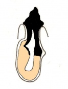
Differentiation of egg cylinder into embryonic and extra-embryonic regions
-Pro-amniotic cavity formation |
Trophoblast giant cells invade maternal tissue
-Maternal blood invades the ectoplacental cone -Reichert's membrane appears -Implantation site is 2x3mm | |
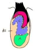
| 9 a) | Pre-streak | Advanced Endometrial and egg cylinder stage
-First evidence of embryonic axis |
Morphological difference can be seen between embryonic and extra-embryonic ectoderm
-Maternal blood further invades ectoplacental cone -Uterine crypts lose their original lumen | |
| 9 b) | Early streak | Gastrulation begins (later in stage) | First mesodermal cells produced | |
| 10 a) | 7 (range 6.5-7.5)
Mid streak to late streak Human carnegie stage: 8 |
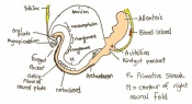
Amnion formation | The amniotic fold starts to form from posterior tissue of primitive streak bulging.
-Allantoic bud evident -Gastrulation continues -Primitive node visible -Amnion begins to close | |
| 11 | 7.5 (range 7.25-8)
Human carnegie stage: 9 |
Formation of neural plate and presomites | Amniotic cavity is sealed to form 3 cavities (amniotic cavity, exocoelom and ectoplacental cleft)
-Allantoic bud elongates -Notochodal plate can be seen in the midline and subjacent to neural groove -Head form from the enlargement of the rostral end of neural plate (early head fold) -Formation of foregut pocket begins |


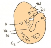
Table 3: Mouse embryonic stages from Theiler stage 15 to 20 ( somite stages)
| Theiler Stage | Embryonic Age (dpc) | Stage Characteristic | Cell Characteristic | Somite Number(pairs | |
|---|---|---|---|---|---|
| 15 | 9.5 (range 9-10.25)
Human carnegie stage: 12 |
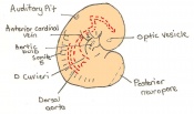
Formation of Forelimb bud
-Posterior neuropore |
8-12th somite pair condensation of forelimb bud is visible
-Hind limb bud appears -Forebrain vesicle division into telencephalic and diencephalic vesicles -Lung development commences -1st sign of Pancreas morphogenesis of dorsal pancreatic bud (22-25 somites). |
21-29 | |
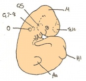
| 16 | 10 (range 9.5-10.75)
Human carnegie stage: 13-15 |
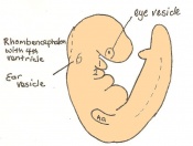
Caudal neuropore closes
-Hind limb bud (23rd-28th somite) and tail bud |
Concave 3rd and 4th branchial arches.
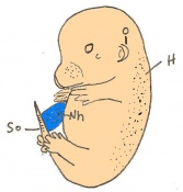
-Rathke's pouch formation -Nasal processes formation. -Ventral pancreatic bud appears |
30-34 | |
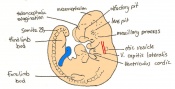
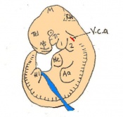
| 17 | 10.5 (range 10-11.25)
Human carnegie stage: 13-15 |
Deep Lens Indentation | Lens pit is deepened and has a narrowed outer opening.
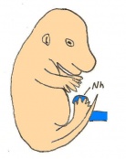
-Physiological umbilical hernia present. -1st branchial arch divides into maxillary and mandibular components. -Advanced development of brain tube -Tail elongates and thins |
35-39 | |
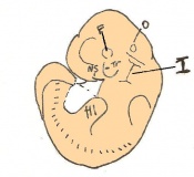
| 18 | 11 (range 10.5-11.25)
Human carnegie stage: 13-15 |
Closure of Lens Vesicle | Cervical somites no longer visible
-Brain rapidly grows -Formation of nasal pit |
40-44 | |
| 19 | 11.5 (range 11-12.25)
Human carnegie stage: 16 |
Lens vesicle separated completely from surface
–Closed and detached from ectoderm |
Well Defined eyes and their peripheral margins
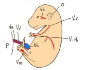
-Forelimbs divided into two regions -Proximal part of the future limb-girdle and 'arm' -Peripheral part forming a circular or anterior footplate. -Otic pit medial and lateral margins move together -Auditory hillocks visible |
45-47 | |
| 20 | 12 (range 11.5-13)
Human carnegie stage: 17 |
First sign of fingers | Anterior footplate no longer circular (develops angles)
-Posterior footplate visible -Pigmentation of retina visible -Tongue and brain vesicles identifiable |
48-51 |
History of the use of the Mouse Embryo Model
Introduction
The mouse has contributed to an important part of research and findings in the biomedical field since the middle of the sixteenth century (Hendrich et al. 2004). In particular, the research of the mouse embryo, has continued into and multiplied within the 20th century.
It's popularity over time in mammalian biology, biomedicine, immunology, oncology, pathology, and genetics is a result of:
- The efficient mouse breeding system: Which consistently monitors the characterisitcs, that are precisley known, generation after generation, thereby producing highly standardised strains (Hedrich et al. 2004).
- The metabolic and internal anatomical similarities between the mouse and the human allows for comparisons. Because of these similarities, they share similar diseases, for example, cancer, diabetes, autoimmunity, endocrine disease, and neurological dysfunctions (Hedrich et al. 2004).
Please note that the following findings are based on research which have utilised the model of the mouse embryo.
1895: Robert Heinrich Johannes Sobotta (1869-1945) [4]
Researched the fertilisation and cleavage of the mouse's egg (Sobotta, 1895). Link to Dr. Sobotta's research [5]
What did he find?
- The corpus Luteum is formed by the enlargement of the epithelial cells of the follicle, aided by growth of connective tissue.
- There is no distinction between corpora lutea vera and corpora lutea spuria.
- The corpora lutea do not degenerate. They remain unchanged during the life of the animal, and therefore add to the size of the ovary.
1958: Professor Dame Anne McLaren
Developed the first birth of mice in-vitro. Link to Published article [6]
1962: George Todaro and Howard Green
- By studying the fibroblast cells of the mouse embryo , they explained how cells behave in a similar fashion once they have undergone transformation (Bhamrah et al. 2002).
How did they do this?
- Todaro and Green cultured the fibroblast cells from the mouse embryo.
What did they find?
- A few weeks after the culture, the growth rate of the Fibroblast cells slowed down. They thought that the cells, as with normal human fibroblast cells, would eventually stop didviding and die. However this was not the case.
- Two to three months later, the cell growth rate increased. This meant that the resulting new population of cells had undergone spontaneous transformation. The resulting permanently dividing cell line, called the '3T3 cell line', have been growing in culture for over 20 years. (Bhamrah et al. 2002)
1977: R.J. Mullen
What did he do?
Fused the normal and reeler mouse embryo at the morula stage to produce allophenic mice. ('The reeler mouse as a model of brain development')
1996: Toshio Ohshima, Jerrold M. Wardt, Chang-Goo Huht, Glenn Longenecker, Veeranna, Harish C.Pant, Roscoe O. Bradyt, Lee J. Martins, and Ashok B. Kulkarni
Generated Cyclin-dependant kinase 5 (Cdk5) null mice (a type of mutant mice) by homologous recombination to assess the role of Cdk5 in vivo. Targeted ES cells were injected into blastocysts to generate chimaric mice
Genetics
Genome
Sequencing of the mouse genome was completed in late 2002. Tha haploid genome is about 3 billion long (3000 Mb distributed over 20 chromosomes) and therefore equal to the size of the human genome. The current estimated gene count is 23,786 and humans are estimated to have 23,686 genes.
The genetic map of the mouse
Genetic maps, the road maps of genetics, are of two types: linkage and physical. The 'sign posts' on the maps are loci, any location or marker in the genome that can be detected by genetic or DNA analysis. The term 'gene' is more restrictive than loci and refers to DNA segments that encode proteins or can be linked to phenotypes. Linkage maps are recombinational maps and are constructed by carrying out linkage crosses that measure the recombination frequency between genes or loci on the same chromosome.
- The first genetic linkage in the mouse (and first autosomal linkage in mammals) was described in 1915 in the classic paper on the linkage of pink-eyed dilution and albino (Haldane et al., 1915)
- Genetic mapping with spontaneous mutations that created visible phenotypes, such as changes in coat colour/texture or behaviour was labarious and sometimes took years because crosses between mice carrying recessive mutations yielded so few informative progeny, and genes on only one or two chromosomes could be scored in each cross.
- The first real breakthrough in linkage mapping, enabling the scoring of many test markers and chromosomes in the same cross, was the discovery and use of co-dominant biochemical (isoenzyme) genes (e.g. glucose phosphate isomerase 1, Gpil; Hutton and Coleman 1969).
How large is the genome?
With the use of Feulgen reagent the quantitative DNA-specific staining can be achieved. Through micro photometric measurements of the staining intensity in individual sperm nuclei, it is possible to determine the total amount of DNA present in the haploid mouse genome (Laird, 1971). Measurements indicated a total haploid genome content of 3 pg, which translates into a molecular weight of 1.8 x 10¹² daltons (Da).
How complex is the genome?
Another method for determining genome size relies upon the kinetics of DNA renaturation as a sign of the total content of different DNA sequences in a sample. When a solution of double stranded DNA is denatured into single strands which are then allowed to renature, the time required for renaturation is directly proportional to the complexity of the DNA in the solution, if all other parameters are held constant.
Complexity is a measure of the information contained within the DNA. The maximal information possible in a solution of genomic DNA purified from one animal or tissue culture line is equivalent to the total number of base pairs present in the haploid genome.The information content of a DNA solution is independent of the actual amount or concentration of DNA present. DNA obtained from one million cells of a single animal or cell line contains no more information than the DNA present in one cell. Furthermore, if sequences within the haploid genome are duplicates of one another — repeated sequences — the complexity will drop accordingly.
Renaturation analysis of mouse DNA reveals an overall complexity of approximately 1.3-1.8 x 10⁹ bp. This value is only 40-60% of the size of the complete haploid genome and it implies the existence of a large fraction of repeated sequences.
Comparative mapping
Comparative mapping began in the early 1970s and gained momentum until it culminated with the sequencing of the two genomes in 2001 and 2002.
- First conserved mouse and human autosomal linkage was reported in 1978.
- 13 conserved autosomal segments and estimated 178(+-)39 chromosomal rearrangements between mouse and human chromosomes were identified (Nadeau and Taylor,1984)
- Sequencing of the two genomes revealed that 95% of the coding sequence is conserved at the DNA level (Consortium,2002)
Current Embryology Research
The mouse is a powerful model organism for research on human disease because it is a mammal and because of the high degree of conservation between the mouse and human genomes.
Knockout Mouse
A knockout mouse is a genetically engineered mouse in which one or more genes have been turned off through a gene knockout. They are important animal models for studying the role of genes which have been sequenced. Mice are currently the most closely related laboratory animal species to humans for which the knockout technique can easily be applied.The first knockout mouse was created by Mario R, Capecchi, Martin Evans and Oliver Smilthies in 1989.
Use
Knocking out the acitivity of a gene provides information about what that gene normally does. Humans share many genes with mice. Consequently, observing the characterisitcs of knockout mice gives researchers information that can be used to better understand how a similar gene may contribute to disease in humans.
Examples of research in which knockout mice have been useful include studying and modeling different kinds of;
- cancer
- obesity
- heart disease
- diabetes
- arthritis
- anxiety
- aging
- Parkinson's disease.
Limitations
While knockout mice technology represents a valuable research tool, some important limitations that exist are;
- About 15% of gene knockouts are developmentally lethal, which means that the genetically altered embryos cannot grow into adult mice. This problem is often overcome through the use of conditional mutations. The lack of adult mice limits studies to embryonic development and often makes it more difficult to determine a gene's function in relation to human health.
- Knocking out a gene may fail to to produce an observable change in a mouse or may even produce different characteristics from those observed in humans in which the same gene is inactivated. E.g mutations in the p53 gene are associated with more than half of human cancers and often lead to tumors in a particular set of tissues. However, when the p53 gene is knocked out in mice, the animals develop tumors in a different array of tissues.
Overview
Mice are highly used models of developmental biology, immunity, neurobiology, and human diseases in pathology. It's main contribution to developmental biology has been through transgenic and knockout technology which are both very important to the research of early development or organogenesis (Slack, 2006).
References
1. Dr Mark Hill 2009, UNSW Embryology ISBN: 978 0 7334 2609 4 - UNSW CRICOS Provider Code No. 00098G [7]
2. Bard, Kaufman, Dubreuil, Brune, Burger, Baldock, Davidson (1998). An internet accessible database of mouse development anatomy based on a systemic nomenclature, Mechanisms of development, (74) 111-120.
3.Hedrich, H., Bullock, G., & Petrusz, P. (2004). The Laboratory Mouse. London: Elsevier Academic Press
4. Theiler, K 1989. 'The House Mouse'. Springer- Verlag, New York
ANAT2341 group projects
Project 1 - Rabbit | Project 2 - Fly | Project 3 - Zebrafish | Group Project 4 - Mouse | Project 5 - Frog | Students Page | Animal Development